Section 3.1 Measures of Central Tendency
¶Definition 3.1.1. Mean (Arithmetic Average).
The mean or arithmetic average is computed by adding up all the values and dividing by the number of observations.
- population mean
\(\mu = \dfrac{\sum x_i}{N}\) (pronounced “mew”)
- sample mean
\(\bar{x} = \dfrac{\sum x_i}{n}\) (pronounced “x bar”)
Note that it is a convention in Statistics to use Greek letters to represent population statistics while we use Roman letters to denote sample statistics.
- Advantage: the mean is used as a starting point for computing several other useful statistics e.g. std. deviation.
- Disadvantage: If the data is skewed or contains outliers, then the mean is not the best way to measure the center of your data.
Definition 3.1.2. Median.
The median or middle value is the value that lies in the middle of the data when the data is arranged in ascending order. Notation: \(M\text{.}\)
Algorithm:
- Sort the data, from least to greatest.
- Find the single middle element, or middle two elements if the list has an even number of elements.
- If there is one value in the middle (\(n\) odd), then that value is the median. If there are two values in the middle (\(n\) even) then the median is the average of the two middle values.
- Advantage: Resistant to outliers and or skewed data.
- Disadvantage: Hard to compute by hand when you have a large data set.
Example 3.1.3. Computing the Median By Hand I.
Find the median of the list: 3, 4, 2, 6, 3.
The ordered list is: 2, 3, 3, 4, 6, and the middle value is 3, thus \(M=3\text{.}\)
Example 3.1.4. Computing the Median By Hand II.
Find the median of the list: 3, 4, 2, 6, 3, 7
The ordered list is: 2, 3, 3, 4, 6, 7, but it has an even number of elements, so we compute the average or mean of the middle two elements, thus the median is:
Definition 3.1.5. Resistant.
A statistic is said to be resistant if extreme values do not affect the value of the statistic.
Definition 3.1.6. Mode.
The mode is the most frequently occurring observation in a data set. A single data set may have multiple modes.
Reading Questions Working Hours
A random sample of 25 college students was asked, “How many hours per week do you typically work outside your home?” Their responses are recorded in the table below.
| 0 | 32 | 15 | 20 | 30 |
| 40 | 30 | 20 | 35 | 35 |
| 28 | 38 | 36 | 25 | 25 |
| 30 | 5 | 28 | 30 | 24 |
| 28 | 30 | 35 | 15 | 32 |
1.
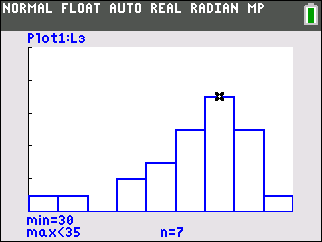
Determine the distribution of the hours worked by creating a frequency histogram on your TI-84 Plus calculator. Use 0 as your lower class limit and 5 as your class width.
First enter the data into any list, press window and enter the following values:
- Xmin=0
- Xmax=45
- Xscl=5
- Ymin=0
- Ymax=10
- Yscl=2
Finally after choosing the correct list in STAT PLOT press graph to plot the histogram with the above settings.
2.
Use your graphing calculator to find the mean and median. Which measure better describes the hours worked?
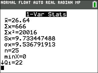
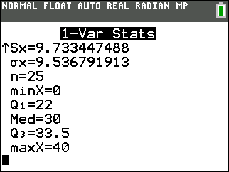
- \(\bar{x} = 26.64\)
- \(M = 30\)
Because the data is skewed to the left, the median is a better measure of the central tendency of the data.