Section 5.1 Probability Rules
¶Definition 5.1.1.
Probability is the measure of the likelihood of a random phenomenon or chance behavior occurring.
It deals with experiments that yield random short-term results or outcomes yet reveal long-term predictability.
The long-term proportion in which a certain outcome is observed is the probability of that outcome.
Fact 5.1.2. Law of Large Numbers.
As the number of repetitions of a probability experiment increases, the proportion of times that a certain outcome is observed gets closer to the probability of the outcome.
Exploration 5.1.1. Simulating Coin Flips on the TI-84 Plus Calculator.
Probability is closely related to performing experiments. However, it is often tedious and time-consuming to perform an experiment by hand. For example, it would be tedious to roll a pair of dice 1000 times and record all the data, but if we program a computer to simulate the experiment we can often get results in a fraction of the time it would take to do the experiment the old fashioned way. Another side benefit of computer simulation is that you can easily share the computer code with others, so they can simulate your experiment as well, and perhaps even improve it.
The following program written in TI-84 BASIC will simulate the flipping of a coin to demonstrate the Law of Large Numbers.
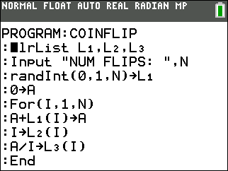
When run (executed), the program does the following:
- Clears lists 1, 2 and 3.
- Prompts you for a number,
N, which is the number of coin flips to perform. - Generates
N, 0's or 1's (pseudo-randomly) and saves the results in list 1. (0=tails, 1=heads) - Initialize an accumulator variable,
A, to 0.Awill keep track of the total number of heads. -
Set
I=1(Ifor “index”) then for each coin flip:- Add the coin value to
A, - Store the value of
Iinto list 2, - Store the current proportion of heads,
A/Iinto list 3.
Increment
Iby 1. Exit the loop ifI > N, otherwise repeat the loop. - Add the coin value to
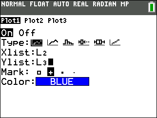
After running the COINFLIP program, you can examine the output it generated by viewing the data in lists 1, 2 and 3. The ideal way to examine the data however is to create a scatter plot using lists 2 and 3. The following STAT PLOT screen shows you how to plot the output of the COINFLIP program.
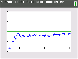
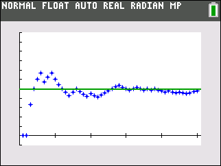
Finally by pressing zoom and then choosing 9:ZoomStat you can generate a plot similar to the two scatter plots below, each of which represents N=50 coin flips. The \(x\)-axis of the scatter plot is the coin flip number, while the \(y\)-axis is the proportion of flips which are heads. Notice that as the number of flips increases the proportion of heads generally gets closer to 0.5 or 50%. This is precisely what the Law of Large Numbers implies.
Before the advent of computers, probability was typically studied in a different way which we will label the “Classical Approach”, as opposed to the experimental or “Empirical Approach” to the study of probability. We will need some new vocabulary in order to discuss the classical approach.
Definition 5.1.5.
The sample space, \(S\text{,}\) of a probability experiment is the collection, or set of all possible outcomes.
An event is any collection of outcomes from a probability experiment. Thus an event is a subset of a sample space. It is common to denote events with capital letters such as \(E, F, G, E_1, E_1, \ldots, E_n\) etc..
Example 5.1.6. Classical and Empirical Comparison.
When you roll a pair of six-sided dice, what is the probability of rolling a five?
Empirical Approach: We could roll a pair of dice say 30 times and record the number of 5's we get. The probability of rolling a 5 on any subsequent roll is then approximated by:
Classical Approach We can enumerate or list all possible outcomes of rolling a pair of dice.
| (1,1) | (1,2) | (1,3) | (1,4) | (1,5) | (1,6) |
| (2,1) | (2,2) | (2,3) | (2,4) | (2,5) | (2,6) |
| (3,1) | (2,2) | (3,3) | (3,4) | (3,5) | (3,6) |
| (4,1) | (4,2) | (4,3) | (4,4) | (4,5) | (4,6) |
| (5,1) | (5,2) | (5,3) | (5,4) | (5,5) | (5,6) |
| (6,1) | (6,2) | (6,3) | (6,4) | (6,5) | (6,6) |
There are exactly 36 possible outcomes all of equal likelihood. Only four of the outcomes: (1,4), (2,3), (3,2), or (4, 1) result in a total of five. Thus since there are four ways to roll a “5”, we get: